Redash is an open-source tool that is available in two versions: self-hosted and cloud. If you use the first one, Redash is free of charge, but for a cloud option you’ll have to pay. In both versions you can connect to a numerous amount of databases (including Clickhouse) or other sources like Google Sheets by API.

Redash is a SQL query editor that allows building visualizations. To make a dashboard, we first need to run a SQL query and then build a visualization. After that, we can add the queries with their visualizations to the dashboard. The process makes data investigations easy and simple.

Data preparation

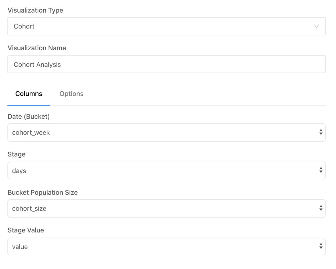
To start working with data we need to click settings and create a new data source.

When working with Superstore dataset we could not directly connect a .xlsx file as redash works only with databases. Thus, we uploaded our .xlsx into a MySQL database.

Building reports and visualizations

In the beginning of the dashboard, you can see the filters. This is the only way to apply filters to a dashboard in Redash and to choose parameters like province interactively.

First of all, we added KPI cards to the dashboard. The functionality of Redash is extremely limited in terms of visualizations, so the only way to build a KPI card was by using so-called counters. A counter is a type of visualization that allows displaying a current and a target value, however, in our case we used the previous year value instead of the target.

For the KPI cards, we used the query below.

It’s a simple query that returns the sum of the profit in current month and the sum of the profit in the previous one. In each query we need to define Year and Month and Province in the WHERE statement, so that all our visualizations are filtered based on the chosen year, month and province. The results are two numbers, curr and prev. Then we click on New Visualization, choose counter as a type and assign curr to the counter value and prev to the target value. We can also change format by adding a dollar sign prefix.

In our previous reviews of BI-tools, we displayed all KPI cards in a single line. In Redash, however, the numbers were too small when displayed in a single line and unnecessary information like the query name and the last update time were cluttering the view. This is another disadvantage of Redash, so we had to make bigger cards and display them in two lines.

To display top performing provinces we used word clouds. The query returned the sum of sales by provinces. Then the sum of sales was used as a frequency column to define the size of the province names.

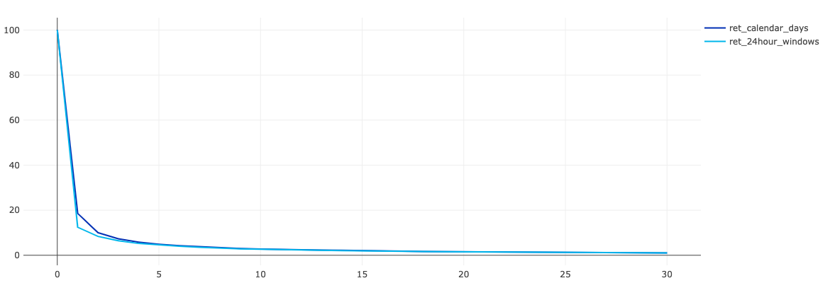
For Profit Dynamics visualization we used a simple line graph. The query below returned a table with total profits for each month as well as two additional columns that display profit in the current month and the previous one.

select date_format(orders.OrderDate, '%Y-%m-01') as month, sum(orders.Profit) as profit, curr.curr_profit, prev.prev_profit
from orders
left join (
    select date_format(OrderDate, '%Y-%m-01') as month, sum(Profit) as curr_profit
    from orders
    where MONTH(OrderDate)=MONTH('{{Year and Month}}') and YEAR(OrderDate)=YEAR('{{Year and Month}}')
        and ('{{Province}}'='0. All' or Province = '{{Province}}')
    group by 1
) curr on curr.month=date_format(orders.OrderDate, '%Y-%m-01')
left join (
    select date_format(OrderDate, '%Y-%m-01') as month, sum(Profit) as prev_profit
    from orders
    where MONTH(OrderDate)=MONTH('{{Year and Month}}') and YEAR(OrderDate)=YEAR('{{Year and Month}}')-1
        and ('{{Province}}'='0. All' or Province = '{{Province}}')
    group by 1
) prev on prev.month=date_format(orders.OrderDate, '%Y-%m-01')
where ('{{Province}}'='0. All' or Province = '{{Province}}')
group by 1,3,4
order by 1

We then used the a line graph to display the profit column and a scatter plot to display curr_profit and prev_profit columns as both of them had only one observation.

Profit and Sales by Category visualization shows a SQL query table that returns profits and sales by category and sub-category of products.

Last but not least, we have pivot tables for top products and top customers by profit. Pivot tables in Redash allow grouping elements by using aggregate functions. In our case we grouped products by profit. I do not recommend using this feature for a large amount of data as if you change the aggregations on the fly in the browser, the browser might slow down and even crash.

Conclusions

You can find the final dashboard here.
Our team has evaluated the dashboard and the following scores on 1-10 scale 10 being the highest were given:

1. Meets the tasks – 7.3
2. Learning curve  – 7.5
3. Tool functionality – 5.5
4. Ease of use – 7.5
5. Compliance with the layout – 6.0
6. Visual evaluation – 5.2

Overall: 6.5 out of 10.

Yesterday I got a message from one of our blog readers, asking:

Let’s say today’s Monday, and an app was downloaded 187 times. If I want to find out what’s the Retention rate was on day 1, what day of the week should I start taking the count with?

He is referring to the blog post on Сalculating Retention Rate. I would like to clarify that since retention rate can be calculated by 24-hour windows, as well as by calendar days. In our case, day 0 will be Monday, and day 1 will be Tuesday. However, there is one little hiccup...

For example, if we started promoting our product on Monday, October 12 at 23:59, then all downloads of this day will have the retention rate of day 1. It’s a problem of performing calendar calculations. To address this, some data analysts calculate retention rate not only by calendar days but also by 24-hour windows.

Let’s apply this idea to the above case:

• The Retention rate for day 0 can be calculated using the number of downloads from October 5, 23:59 to October 6, 23:59.
• The Retention rate for day 1: from October 6, 23:59 to October 7, 23:59
• And so on rolling 24-hour window.

How to calculate Retention Rate by 24-hour windows in SQL?

Let’s recall one of the queries from our previous post. It was written to calculate the difference between the download date and the user activity date. We need to change the query so that user activity is calculated by 24-hour windows. To accomplish this just change the calculation for datediff to 24-hour windows, updating the lines in bold.

SELECT from_unixtime(user.installed_at, "yyyy-MM-dd") AS reg_date,
   floor((cast(cs.created_at as int)-cast(installed_at as int))/(24*3600)) as date_diff,
   ndv(user.id) AS ret_base
   FROM USER
   LEFT JOIN client_session cs ON cs.user_id=user.id
   WHERE 1=1
     AND floor((cast(cs.created_at as int)-cast(installed_at as int))/(24*3600)) between 0 and 30
     AND from_unixtime(user.installed_at)>=date_add(now(), -60)
     AND from_unixtime(user.installed_at)<=date_add(now(), -31)
   GROUP BY 1,2

Updated query:

SELECT 
       cohort.date_diff AS day_difference,
       avg(reg.users) AS cohort_size,
       avg(cohort.ret_base) AS retention_base,
       avg(cohort.ret_base)/avg(reg.users)*100 AS retention_rate
FROM
  (SELECT from_unixtime(user.installed_at, "yyyy-MM-dd") AS reg_date,
          ndv(user.id) AS users
   FROM USER
   WHERE from_unixtime(user.installed_at)>=date_add(now(), -60)
     AND from_unixtime(user.installed_at)<=date_add(now(), -31)
   GROUP BY 1) reg
LEFT JOIN
  (SELECT from_unixtime(user.installed_at, "yyyy-MM-dd") AS reg_date,
    floor((cast(cs.created_at as int)-cast(installed_at as int))/(24*3600)) as date_diff,
          ndv(user.id) AS ret_base
   FROM USER
   LEFT JOIN client_session cs ON cs.user_id=user.id
    WHERE 1=1
     AND floor((cast(cs.created_at as int)-cast(installed_at as int))/(24*3600)) between 0 and 30
     AND from_unixtime(user.installed_at)>=date_add(now(), -60)
     AND from_unixtime(user.installed_at)<=date_add(now(), -31)
   GROUP BY 1,2
  ) cohort ON reg.reg_date=cohort.reg_date
    GROUP BY 1        
    ORDER BY 1

Final output:

Compare it with the previous one:

And as you see, the retention rate calculated using 24-hour windows is slightly lower in the first days.

In our new series, we will try to give a detailed representation of  several BI tools using the SuperStore Sales dataset. The data in SuperStore Sales reflect sales and profit of the retail chain in US dollars.

In the upcoming blog post, we will discuss a real problem statement that could arise when creating a dashboard based on the SuperStore Sales data and design a functional layout to provide clear answers. Throughout this task, we’ll stick with a predefined set of colors to make the comparison more unbiased.

Next, we’re going to create a dashboard that would assist in data-based decision-making with each of the BI tools. We also plan to involve industry experts to learn from their experience.

A complete list of BI systems and tools to be tested in our experiment is provided below. I want to welcome everyone who is willing to help us in solving this challenge to message me on Telegram  – @valiotti. I will be glad to hear from you. Although it’s a non-profit project, it’ll be really useful for the open-source community.

We plan to cover the following list of tools:

Free Open Source:

• Metabase
• Redash
• Apache Superset
• Dash / Plotly

Free Cloud-Based:

• Google Studio
• Yandex Datalens

Paid Cloud-Based:

• Mode
• Cluvio
• Holistic
• Chartio
• Periscope
• DeltaDNA
• Klipfolio
• Count.co

Paid:

• PowerBI
• Tableau
• Looker
• Excel
• Alteryx
• Qlik Sense
• Qlik View

The final goal is to evaluate the BI tools against the following criteria:

• learning curve of BI tool (1 — too hard to learn, 10 — easy)
• tool functionality (1 — very poor functionality, 10 — multifunctional)
• ease of use (1 — very inconvenient, 10 — super convenient)
• compliance of the result (1 — far from the designed layout, 10 — too close to the designed layout and objective)
• visual evaluation (1 — poor appearance, 10 — great visual appearance)

An integral weighted score for each tool will be calculated based on the internal estimates.

The results will be posted to our Telegram channel @leftjoin_en and followers will also be able to share their thoughts on the experiment.
By the end, each tool will be represented as a point in the plane, which will be divided into 4 parts.

This article will be updated with links and ratings as we new posts come out.

Our previous article was dedicated to collecting data on Facebook ad campaigns. Today we will analyze this data using Redash. As a first step, we need to upload our script to AWS cloud and create a server with AIOHTTP before passing the data to Redash. Let’s improve the script a little bit for this task:

from facebook_business.api import FacebookAdsApi
from facebook_business.adobjects.adaccount import AdAccount
from facebook_business.adobjects.adreportrun import AdReportRun
from facebook_business.adobjects.adsinsights import AdsInsights
from facebook_business.adobjects.adaccountuser import AdAccountUser as AdUser
from facebook_business.exceptions import FacebookRequestError
import time

Redash receives data in JSON format, which we haven’t covered yet. A JSON file is a file that consists of a list of dictionaries. The script will convert it to JSON and pass the data to Redash. We’ll need the variable that stores our access token, app id, app secret and two functions: wait_for_async_job() and get_insights(). The latter function receives account parameters and collects data on ad campaigns. Select the following fields: clicks, impressions, costs and dates.

We need the entire script from our previous article – “Collecting Data on Facebook Ad Campaigns”

The return_json() function will call the get_insights(), which will append data to insights_lists. Since we may have several ad campaigns, our output can be a list of lists with dictionaries instead of just a list of dictionaries. Create a simple lambda expression that will smooth the output and return our insights_lists_flatten. Now, the script returns a list of dictionaries:

def return_json():
   insights_lists = []
   date_preset = 'last_year'
   for elem in my_accounts:
       elem_insights = get_insights(elem, date_preset)
       insights_lists.append(elem_insights)
   flatten = lambda lst: [item for sublist in lst for item in sublist]
   insights_lists_flatten = flatten(insights_lists)
   return insights_lists_flatten

We also need a AIOHTTP server that will return our output as JSON. Create a new file, import the AIOHTTP library and the get_json() function from the preceding script. Write a simple query handler: the script will receive data from Facebook asynchronously and our asynchronous handler function will sleep until all data is collected and transferred. The function uses json_response to transfer data in json format.

from aiohttp import web
from get_json import return_json

async def handler(request):
   data = return_json()
   return web.json_response(data)

Initialize and run our application.

app = web.Application()
app.add_routes([web.get('/json', handler)])
web.run_app(app)

Now, go to AWS cloud, create a new folder and upload the two scripts via SFTP connection. Check if the needed port is open, click console — network & security — security groups — default.

Run our file from the server. You can check whether it works by accessing it via server IP address specifying 0880 in the route field. Connect to Redash using URL and we’ll get the same table returned by our script:

url: server ip

Having query results, we can write the following query:

select date_start, sum(clicks) as clicks, sum(impressions) as impressions, sum(spend) as spend from query_45
group by date_start

It returns this table, grouped by the date_start column:

We can now plot this data on the chart, let’s see if there is any correlation between ad costs and clicks:

Bingo! Next time, we will show you how to get data on ad campaigns from Vkontakte.

In one of the previous articles we have reviewed building of Retention-report and have partially addressed the concept of cohorts therein.
Cohort usually implies group of users of a product or a company. Most often, groups are allocated on the basis of time of app installation / appearance of a user in a system.
It turns out, that, using cohort analysis, one can track down how the changes in a product affected the behaviour of users (for example, of old and new users).

Along with that, cohorts can be defined also proceeding from other parameters: geography of a user, traffic source, device platform and other important parameters of your product.

We will figure out, how to compare Retention of users of weekly cohorts in Redash, since Redash has special type of visualization for building such type of report.
Firstly, let’s sort out SQL-query. We still have two tables – user (id of a user and time of app installation) and client_session – timestamps (created_at) of activity of each user (user_id). Let’s consider the Retention of the first seven days for last 60 days.
The query is written in Cloudera Impala, let’s review it.

For starters, let’s build the total size of cohorts:

select trunc(from_unixtime(user.installed_at), "WW") AS cohort_week, 
	ndv(distinct user.id) as cohort_size //counting the number of users in the cohort
	from user 
	where from_unixtime(user.installed_at) between date_add(now(), -60) and now() //taking registered users for last 60 days
group by trunc(from_unixtime(user.installed_at), "WW")

The second part of the query can calculate the quantity of active users for every day during the first thirty days:

select trunc(from_unixtime(user.installed_at), "WW") AS cohort_week, 
        datediff(cast(cs.created_at as timestamp),cast(user.installed_at as timestamp)) as days,
	ndv(distinct user.id) as value  //counting the number of active users for every day
		from user 
		left join client_session cs on user.id=cs.user_id
where from_unixtime(user.installed_at) between date_add(now(), -60) and now()
and from_unixtime(cs.created_at) >= date_add(now(), -60) //taking sessions for last 60 days
and datediff(cast(cs.created_at as timestamp),cast(user.installed_at as timestamp)) between 0 and 30 //cutting off only the first 30 days of activity
group by 1,2

Bottom line, all the query entirely:

select size.cohort_week, size.cohort_size, ret.days, ret.value from
(select trunc(from_unixtime(user.installed_at), "WW") AS cohort_week, 
		ndv(distinct user.id) as cohort_size 
	from user 
	where from_unixtime(user.installed_at) between date_add(now(), -60) and now()
group by trunc(from_unixtime(user.installed_at), "WW")) size
left join (select trunc(from_unixtime(user.installed_at), "WW") AS cohort_week, 
        datediff(cast(cs.created_at as timestamp),cast(user.installed_at as timestamp)) as days,
		ndv(distinct user.id) as value 
		from user 
		left join client_session cs on user.id=cs.user_id
where from_unixtime(user.installed_at) between date_add(now(), -60) and now()
and from_unixtime(cs.created_at) >= date_add(now(), -60)
and datediff(cast(cs.created_at as timestamp),cast(user.installed_at as timestamp)) between 0 and 30
group by 1,2) ret on size.cohort_week=ret.cohort_week

Great, now correctly calculated data is available to us.

Data of cohorts in tabular form

Let’s create new visualization in Redash and indicate the parameters correctly:

It’s important to indicate the parameters correctly – the columns of the resulting query are compliant therewith.

Let’s make sure to indicate that we have weekly cohorts:

Voila, our visualization of cohorts is ready:

You can add filters and parameters to it and use in a dashboard

Materials on the topic

• Cohort analysis. Metrics of product vs metrics of growth
• A beginners guide to cohort analysis