In one of the previous articles we have reviewed building of Retention-report and have partially addressed the concept of cohorts therein.
Cohort usually implies group of users of a product or a company. Most often, groups are allocated on the basis of time of app installation / appearance of a user in a system.
It turns out, that, using cohort analysis, one can track down how the changes in a product affected the behaviour of users (for example, of old and new users).

Along with that, cohorts can be defined also proceeding from other parameters: geography of a user, traffic source, device platform and other important parameters of your product.

We will figure out, how to compare Retention of users of weekly cohorts in Redash, since Redash has special type of visualization for building such type of report.
Firstly, let’s sort out SQL-query. We still have two tables – user (id of a user and time of app installation) and client_session – timestamps (created_at) of activity of each user (user_id). Let’s consider the Retention of the first seven days for last 60 days.
The query is written in Cloudera Impala, let’s review it.

For starters, let’s build the total size of cohorts:

select trunc(from_unixtime(user.installed_at), "WW") AS cohort_week, 
	ndv(distinct user.id) as cohort_size //counting the number of users in the cohort
	from user 
	where from_unixtime(user.installed_at) between date_add(now(), -60) and now() //taking registered users for last 60 days
group by trunc(from_unixtime(user.installed_at), "WW")

The second part of the query can calculate the quantity of active users for every day during the first thirty days:

select trunc(from_unixtime(user.installed_at), "WW") AS cohort_week, 
        datediff(cast(cs.created_at as timestamp),cast(user.installed_at as timestamp)) as days,
	ndv(distinct user.id) as value  //counting the number of active users for every day
		from user 
		left join client_session cs on user.id=cs.user_id
where from_unixtime(user.installed_at) between date_add(now(), -60) and now()
and from_unixtime(cs.created_at) >= date_add(now(), -60) //taking sessions for last 60 days
and datediff(cast(cs.created_at as timestamp),cast(user.installed_at as timestamp)) between 0 and 30 //cutting off only the first 30 days of activity
group by 1,2

Bottom line, all the query entirely:

select size.cohort_week, size.cohort_size, ret.days, ret.value from
(select trunc(from_unixtime(user.installed_at), "WW") AS cohort_week, 
		ndv(distinct user.id) as cohort_size 
	from user 
	where from_unixtime(user.installed_at) between date_add(now(), -60) and now()
group by trunc(from_unixtime(user.installed_at), "WW")) size
left join (select trunc(from_unixtime(user.installed_at), "WW") AS cohort_week, 
        datediff(cast(cs.created_at as timestamp),cast(user.installed_at as timestamp)) as days,
		ndv(distinct user.id) as value 
		from user 
		left join client_session cs on user.id=cs.user_id
where from_unixtime(user.installed_at) between date_add(now(), -60) and now()
and from_unixtime(cs.created_at) >= date_add(now(), -60)
and datediff(cast(cs.created_at as timestamp),cast(user.installed_at as timestamp)) between 0 and 30
group by 1,2) ret on size.cohort_week=ret.cohort_week

Great, now correctly calculated data is available to us.

Data of cohorts in tabular form

Let’s create new visualization in Redash and indicate the parameters correctly:

It’s important to indicate the parameters correctly – the columns of the resulting query are compliant therewith.

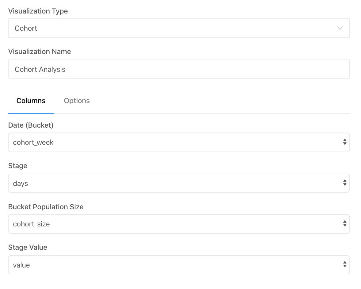
Let’s make sure to indicate that we have weekly cohorts:

Voila, our visualization of cohorts is ready:

You can add filters and parameters to it and use in a dashboard

Materials on the topic

• Cohort analysis. Metrics of product vs metrics of growth
• A beginners guide to cohort analysis