Hans Rosling’s work on world countries economic growth presented in 2007 at TEDTalks can be attributed to one of the most iconic data visualizations, ever created. Just check out this video, in case you don’t know what we’re talking about:

Sometimes we want to compare standards of living in other countries. One way to do this is to refer to the Big Mac index, which the Economist magazine has kept track of since 1986. The key idea this index represents is to measure purchasing power parity (PPP) in different countries, considering costs of domestic production. To make a standard burger, one would need the following ingredients: cheese, meat, bread and vegetables. Considering that all these ingredients can be produced locally, we can compare the production cost of one Big Mac in different countries, and measure purchasing power. Plus, McDonald’s is the world’s most popular franchise network, its restaurants are almost everywhere around the globe.

In today’s material, we will build a Motion Chart for the Big Mac index using Plotly. Following Hann Rosling’s idea, the chart will display country population along the X-axis and GDP per capita in US dollars along the Y. The size of the dots is going to be proportional to the Big Mac Index for a given country. And the color of the dots will represent the continent where the country is located.

Preparing Data

Even though The Economist has been updating it for over 30 years and sharing its observations publicly, the dataset contains many missing values. It also lacks continents names, but we can handle it by supplementing the data with some more datasets that can be found in our repo.

Let’s start by importing the libraries:

import pandas as pd
from pandas.errors import ParserError
import plotly.graph_objects as go
import numpy as np
import requests
import io

We can access the dataset directly from GitHub. Just use the following function to send a GET request to a CSV file and create a Pandas DataFrame. However, in some cases, this may raise a  ParseError because of the caption title, so we will add a try block:

def read_raw_file(link):
    raw_csv = requests.get(link).content
    try:
        df = pd.read_csv(io.StringIO(raw_csv.decode('utf-8')))
    except ParserError:
        df = pd.read_csv(io.StringIO(raw_csv.decode('utf-8')), skiprows=3)
    return df

bigmac_df = read_raw_file('https://github.com/valiotti/leftjoin/raw/master/motion-chart-big-mac/big-mac.csv')
population_df = read_raw_file('https://github.com/valiotti/leftjoin/raw/master/motion-chart-big-mac/population.csv')
dgp_df = read_raw_file('https://github.com/valiotti/leftjoin/raw/master/motion-chart-big-mac/gdp.csv')
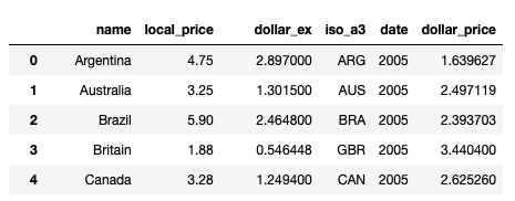
continents_df = read_raw_file('https://github.com/valiotti/leftjoin/raw/master/motion-chart-big-mac/continents.csv')

From The Economist dataset we will need these columns: country name, local price, dollar exchange rate, country code (iso_a3) and record date. Take the timeline from 2005 to 2020, as the records are most complete for this span. And divide the local price by the exchange rate to calculate the price of one Big Mac in US dollars.

bigmac_df = bigmac_df[['name', 'local_price', 'dollar_ex', 'iso_a3', 'date']]
bigmac_df = bigmac_df[bigmac_df['date'] >= '2005-01-01']
bigmac_df = bigmac_df[bigmac_df['date'] < '2020-01-01']
bigmac_df['date'] = pd.DatetimeIndex(bigmac_df['date']).year
bigmac_df = bigmac_df.drop_duplicates(['date', 'name'])
bigmac_df = bigmac_df.reset_index(drop=True)
bigmac_df['dollar_price'] = bigmac_df['local_price'] / bigmac_df['dollar_ex']

Take a look at the result:

Next, let’s try adding a new column called continents. To ease the task, leave only two columns containing country code and continent name. Then we need to iterate through the bigmac_df[‘iso_a3’] column, adding a continent name for the corresponding values. However some cases may raise an error, because it’s not really clear, whether a country belongs to Europe or Asia, we will consider such cases as Europe by default.

continents_df = continents_df[['Continent_Name', 'Three_Letter_Country_Code']]
continents_list = []
for country in bigmac_df['iso_a3']:
    try:
        continents_list.append(continents_df.loc[continents_df['Three_Letter_Country_Code'] == country]['Continent_Name'].item())
    except ValueError:
        continents_list.append('Europe')
bigmac_df['continent'] = continents_list

Now we can drop unnecessary columns, apply sorting by country names and date, convert values in the date column into integers, and view the current result:

bigmac_df = bigmac_df.drop(['local_price', 'iso_a3', 'dollar_ex'], axis=1)
bigmac_df = bigmac_df.sort_values(by=['name', 'date'])
bigmac_df['date'] = bigmac_df['date'].astype(int)

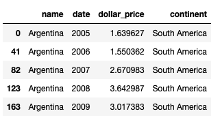
Then we need to fill up missing values for The Big Mac index with zeros and remove the Republic of China, since this partially recognized state is not included in the World Bank datasets. The UAE occurs several times, this can lead to issues.

countries_list = list(bigmac_df['name'].unique())
years_set = {i for i in range(2005, 2020)}
for country in countries_list:
    if len(bigmac_df[bigmac_df['name'] == country]) < 15:
        this_continent = bigmac_df[bigmac_df['name'] == country].continent.iloc[0]
        years_of_country = set(bigmac_df[bigmac_df['name'] == country]['date'])
        diff = years_set - years_of_country
        dict_to_df = pd.DataFrame({
                      'name':[country] * len(diff),
                      'date':list(diff),
                      'dollar_price':[0] * len(diff),
                      'continent': [this_continent] * len(diff)
                     })
        bigmac_df = bigmac_df.append(dict_to_df)
bigmac_df = bigmac_df[bigmac_df['name'] != 'Taiwan']
bigmac_df = bigmac_df[bigmac_df['name'] != 'United Arab Emirates']

Next, let’s augment the data with GDP per capita and population from other datasets. Both datasets have differences in country names, so we need to specify such cases explicitly and replace them.

years = [str(i) for i in range(2005, 2020)]

countries_replace_dict = {
    'Russian Federation': 'Russia',
    'Egypt, Arab Rep.': 'Egypt',
    'Hong Kong SAR, China': 'Hong Kong',
    'United Kingdom': 'Britain',
    'Korea, Rep.': 'South Korea',
    'United Arab Emirates': 'UAE',
    'Venezuela, RB': 'Venezuela'
}
for key, value in countries_replace_dict.items():
    population_df['Country Name'] = population_df['Country Name'].replace(key, value)
    gdp_df['Country Name'] = gdp_df['Country Name'].replace(key, value)

Finally, extract population data and GDP for the given years, adding the data to the bigmac_df DataFrame:

countries_list = list(bigmac_df['name'].unique())

population_list = []
gdp_list = []
for country in countries_list:
    population_for_country_df = population_df[population_df['Country Name'] == country][years]
    population_list.extend(list(population_for_country_df.values[0]))
    gdp_for_country_df = gdp_df[gdp_df['Country Name'] == country][years]
    gdp_list.extend(list(gdp_for_country_df.values[0]))
    
bigmac_df['population'] = population_list
bigmac_df['gdp'] = gdp_list
bigmac_df['gdp_per_capita'] = bigmac_df['gdp'] / bigmac_df['population']

And here is our final dataset:

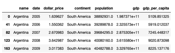
Creating a chart in Plotly

The population in China or India, on average, is 10 times more than in other countries. That’s why we need to transform X-axis to Log Scale, to make the chart easier for interpreting. The log-transformation is a common way to address skewness in data.

fig_dict = {
    "data": [],
    "layout": {},
    "frames": []
}

fig_dict["layout"]["xaxis"] = {"title": "Population", "type": "log"}
fig_dict["layout"]["yaxis"] = {"title": "GDP per capita (in $)", "range":[-10000, 120000]}
fig_dict["layout"]["hovermode"] = "closest"
fig_dict["layout"]["updatemenus"] = [
    {
        "buttons": [
            {
                "args": [None, {"frame": {"duration": 500, "redraw": False},
                                "fromcurrent": True, "transition": {"duration": 300,
                                                                    "easing": "quadratic-in-out"}}],
                "label": "Play",
                "method": "animate"
            },
            {
                "args": [[None], {"frame": {"duration": 0, "redraw": False},
                                  "mode": "immediate",
                                  "transition": {"duration": 0}}],
                "label": "Pause",
                "method": "animate"
            }
        ],
        "direction": "left",
        "pad": {"r": 10, "t": 87},
        "showactive": False,
        "type": "buttons",
        "x": 0.1,
        "xanchor": "right",
        "y": 0,
        "yanchor": "top"
    }
]

We will also add a slider to filter data within a certain range:

sliders_dict = {
    "active": 0,
    "yanchor": "top",
    "xanchor": "left",
    "currentvalue": {
        "font": {"size": 20},
        "prefix": "Year: ",
        "visible": True,
        "xanchor": "right"
    },
    "transition": {"duration": 300, "easing": "cubic-in-out"},
    "pad": {"b": 10, "t": 50},
    "len": 0.9,
    "x": 0.1,
    "y": 0,
    "steps": []
}

By default, the chart will display data for 2005 before we click on the “Play” button.

continents_list_from_df = list(bigmac_df['continent'].unique())
year = 2005
for continent in continents_list_from_df:
    dataset_by_year = bigmac_df[bigmac_df["date"] == year]
    dataset_by_year_and_cont = dataset_by_year[dataset_by_year["continent"] == continent]
    
    data_dict = {
        "x": dataset_by_year_and_cont["population"],
        "y": dataset_by_year_and_cont["gdp_per_capita"],
        "mode": "markers",
        "text": dataset_by_year_and_cont["name"],
        "marker": {
            "sizemode": "area",
            "sizeref": 200000,
            "size":  np.array(dataset_by_year_and_cont["dollar_price"]) * 20000000
        },
        "name": continent,
        "customdata": np.array(dataset_by_year_and_cont["dollar_price"]).round(1),
        "hovertemplate": '<b>%{text}</b>' + '<br>' +
                         'GDP per capita: %{y}' + '<br>' +
                         'Population: %{x}' + '<br>' +
                         'Big Mac price: %{customdata}$' +
                         '<extra></extra>'
    }
    fig_dict["data"].append(data_dict)

Next, we need to fill up the frames field, which will be used for animating the data. Each frame represents a certain data point from 2005 to 2019.

for year in years:
    frame = {"data": [], "name": str(year)}
    for continent in continents_list_from_df:
        dataset_by_year = bigmac_df[bigmac_df["date"] == int(year)]
        dataset_by_year_and_cont = dataset_by_year[dataset_by_year["continent"] == continent]

        data_dict = {
            "x": list(dataset_by_year_and_cont["population"]),
            "y": list(dataset_by_year_and_cont["gdp_per_capita"]),
            "mode": "markers",
            "text": list(dataset_by_year_and_cont["name"]),
            "marker": {
                "sizemode": "area",
                "sizeref": 200000,
                "size": np.array(dataset_by_year_and_cont["dollar_price"]) * 20000000
            },
            "name": continent,
            "customdata": np.array(dataset_by_year_and_cont["dollar_price"]).round(1),
            "hovertemplate": '<b>%{text}</b>' + '<br>' +
                             'GDP per capita: %{y}' + '<br>' +
                             'Population: %{x}' + '<br>' +
                             'Big Mac price: %{customdata}$' +
                             '<extra></extra>'
        }
        frame["data"].append(data_dict)

    fig_dict["frames"].append(frame)
    slider_step = {"args": [
        [year],
        {"frame": {"duration": 300, "redraw": False},
         "mode": "immediate",
         "transition": {"duration": 300}}
    ],
        "label": year,
        "method": "animate"}
    sliders_dict["steps"].append(slider_step)

Just a few finishing touches left, instantiate the chart, set colors, fonts and title.

fig_dict["layout"]["sliders"] = [sliders_dict]

fig = go.Figure(fig_dict)

fig.update_layout(
    title = 
        {'text':'<b>Motion chart</b><br><span style="color:#666666">The Big Mac index from 2005 to 2019</span>'},
    font={
        'family':'Open Sans, light',
        'color':'black',
        'size':14
    },
    plot_bgcolor='rgba(0,0,0,0)'
)
fig.update_yaxes(nticks=4)
fig.update_xaxes(tickfont=dict(family='Open Sans, light', color='black', size=12), nticks=4, gridcolor='lightgray', gridwidth=0.5)
fig.update_yaxes(tickfont=dict(family='Open Sans, light', color='black', size=12), nticks=4, gridcolor='lightgray', gridwidth=0.5)

fig.show()

Bingo! The Motion Chart is done:

View the code on GitHub

Instagram is in the top 5 most visited websites, perhaps not for our industry. Nevertheless, we are going to test this hypothesis using Python and our data analytics skills. In this post, we will share how to collect social media data using the Instagram API.

Data collection method
The Instagram API won’t let us collect data about other platform users for no reason, but there is always a way. Try sending the following request:

https://instagram.com/leftjoin/?__a=1

The request returns a JSON object with detailed user information, for instance, we can easily get an account name, number of posts, followers, subscriptions, as well as the first ten user posts with likes count, comments and etc. The pyInstagram library allows sending such requests.

SQL schema
Data will be collected into thee Clickhouse tables: users, posts, comments. The users table will contain user data, such as user id, username, user’s first and last name, account description, number of followers, subscriptions, posts, comments, and likes, whether an account is verified or not, and so on.

CREATE TABLE instagram.users
(
    `added_at` DateTime,
    `user_id` UInt64,
    `user_name` String,
    `full_name` String,
    `base_url` String,
    `biography` String,
    `followers_count` UInt64,
    `follows_count` UInt64,
    `media_count` UInt64,
    `total_comments` UInt64,
    `total_likes` UInt64,
    `is_verified` UInt8,
    `country_block` UInt8,
    `profile_pic_url` Nullable(String),
    `profile_pic_url_hd` Nullable(String),
    `fb_page` Nullable(String)
)
ENGINE = ReplacingMergeTree
ORDER BY added_at

The posts table will be populated with the post owner name, post id, caption, comments coun, and so on. To check whether a post is an advertisement, Instagram carousel, or a video we can use these fields: is_ad, is_album and is_video.

CREATE TABLE instagram.posts
(
    `added_at` DateTime,
    `owner` String,
    `post_id` UInt64,
    `caption` Nullable(String),
    `code` String,
    `comments_count` UInt64,
    `comments_disabled` UInt8,
    `created_at` DateTime,
    `display_url` String,
    `is_ad` UInt8,
    `is_album` UInt8,
    `is_video` UInt8,
    `likes_count` UInt64,
    `location` Nullable(String),
    `recources` Array(String),
    `video_url` Nullable(String)
)
ENGINE = ReplacingMergeTree
ORDER BY added_at

In the comments table, we store each comment separately with the comment owner and text.

CREATE TABLE instagram.comments
(
    `added_at` DateTime,
    `comment_id` UInt64,
    `post_id` UInt64,
    `comment_owner` String,
    `comment_text` String
)
ENGINE = ReplacingMergeTree
ORDER BY added_at

Writing the script
Import the following classes from the library: Account, Media, WebAgent and Comment.

from instagram import Account, Media, WebAgent, Comment
from datetime import datetime
from clickhouse_driver import Client
import requests
import pandas as pd

Next, create an instance of the WebAgent class required for some library methods and data updating. To collect any meaningful information we need to have at least account names. Since we don’t have them yet, send the following request to search for porifles by the  keywords specified in queries_list. The search results will be composed of Instagram pages that match any keyword in the list.

agent = WebAgent()
queries_list = ['machine learning', 'data science', 'data analytics', 'analytics', 'business intelligence',
                'data engineering', 'computer science', 'big data', 'artificial intelligence',
                'deep learning', 'data scientist','machine learning engineer', 'data engineer']
client = Client(host='12.34.56.789', user='default', password='', port='9000', database='instagram')
url = 'https://www.instagram.com/web/search/topsearch/?context=user&count=0'

Let’s iterate the keywords collecting all matching accounts. Then remove duplicates from the obtained list by converting it to set and back.

response_list = []
for query in queries_list:
    response = requests.get(url, params={
        'query': query
    }).json()
    response_list.extend(response['users'])
instagram_pages_list = []
for item in response_list:
    instagram_pages_list.append(item['user']['username'])
instagram_pages_list = list(set(instagram_pages_list))

Now we need to loop through the list of pages and request detailed information about an account if it’s not in the table yet. Create an instance of the Account class and pass username as a parameter.
Then update the account information using the agent.update()
method. We will collect only the first 100 posts to keep it moving. Next, create a list named media_list to store received post ids after calling the agent.get_media() method.

all_posts_list = []
username_count = 0
for username in instagram_pages_list:
    if client.execute(f"SELECT count(1) FROM users WHERE user_name='{username}'")[0][0] == 0:
        print('username:', username_count, '/', len(instagram_pages_list))
        username_count += 1
        account_total_likes = 0
        account_total_comments = 0
        try:
            account = Account(username)
        except Exception as E:
            print(E)
            continue
        try:
            agent.update(account)
        except Exception as E:
            print(E)
            continue
        if account.media_count < 100:
            post_count = account.media_count
        else:
            post_count = 100
        print(account, post_count)
        media_list, _ = agent.get_media(account, count=post_count, delay=1)
        count = 0

Because we need to count the total number of likes and comments before adding a new user to our database, we’ll start with them first. Almost all required fields belong to the Media class:

for media_code in media_list:
            if client.execute(f"SELECT count(1) FROM posts WHERE code='{media_code}'")[0][0] == 0:
                print('posts:', count, '/', len(media_list))
                count += 1

                post_insert_list = []
                post = Media(media_code)
                agent.update(post)
                post_insert_list.append(datetime.now().strftime('%Y-%m-%d %H:%M:%S'))
                post_insert_list.append(str(post.owner))
                post_insert_list.append(post.id)
                if post.caption is not None:
                    post_insert_list.append(post.caption.replace("'","").replace('"', ''))
                else:
                    post_insert_list.append("")
                post_insert_list.append(post.code)
                post_insert_list.append(post.comments_count)
                post_insert_list.append(int(post.comments_disabled))
                post_insert_list.append(datetime.fromtimestamp(post.date).strftime('%Y-%m-%d %H:%M:%S'))
                post_insert_list.append(post.display_url)
                try:
                    post_insert_list.append(int(post.is_ad))
                except TypeError:
                    post_insert_list.append('cast(Null as Nullable(UInt8))')
                post_insert_list.append(int(post.is_album))
                post_insert_list.append(int(post.is_video))
                post_insert_list.append(post.likes_count)
                if post.location is not None:
                    post_insert_list.append(post.location)
                else:
                    post_insert_list.append('')
                post_insert_list.append(post.resources)
                if post.video_url is not None:
                    post_insert_list.append(post.video_url)
                else:
                    post_insert_list.append('')
                account_total_likes += post.likes_count
                account_total_comments += post.comments_count
                try:
                    client.execute(f'''
                        INSERT INTO posts VALUES {tuple(post_insert_list)}
                    ''')
                except Exception as E:
                    print('posts:')
                    print(E)
                    print(post_insert_list)

Store comments in the variable with the same name after calling the get_comments() method:

comments = agent.get_comments(media=post)
                for comment_id in comments[0]:
                    comment_insert_list = []
                    comment = Comment(comment_id)
                    comment_insert_list.append(datetime.now().strftime('%Y-%m-%d %H:%M:%S'))
                    comment_insert_list.append(comment.id)
                    comment_insert_list.append(post.id)
                    comment_insert_list.append(str(comment.owner))
                    comment_insert_list.append(comment.text.replace("'","").replace('"', ''))
                    try:
                        client.execute(f'''
                            INSERT INTO comments VALUES {tuple(comment_insert_list)}
                        ''')
                    except Exception as E:
                        print('comments:')
                        print(E)
                        print(comment_insert_list)

And now, when we have obtained user posts and comments new information can be added to the table.

user_insert_list = []
        user_insert_list.append(datetime.now().strftime('%Y-%m-%d %H:%M:%S'))
        user_insert_list.append(account.id)
        user_insert_list.append(account.username)
        user_insert_list.append(account.full_name)
        user_insert_list.append(account.base_url)
        user_insert_list.append(account.biography)
        user_insert_list.append(account.followers_count)
        user_insert_list.append(account.follows_count)
        user_insert_list.append(account.media_count)
        user_insert_list.append(account_total_comments)
        user_insert_list.append(account_total_likes)
        user_insert_list.append(int(account.is_verified))
        user_insert_list.append(int(account.country_block))
        user_insert_list.append(account.profile_pic_url)
        user_insert_list.append(account.profile_pic_url_hd)
        if account.fb_page is not None:
            user_insert_list.append(account.fb_page)
        else:
            user_insert_list.append('')
        try:
            client.execute(f'''
                INSERT INTO users VALUES {tuple(user_insert_list)}
            ''')
        except Exception as E:
            print('users:')
            print(E)
            print(user_insert_list)

Conclusion
To sum up, we have collected data of 500 users, with nearly 20K posts and 40K comments. As the database will be updated, we can write a simple query to get the top 10 ML, AI & Data Science related most followed accounts for today.

SELECT *
FROM users
ORDER BY followers_count DESC
LIMIT 10

And as a bonus, here is a list of the most interesting Instagram accounts on this topic:

1. @ai_machine_learning
2. @neuralnine
3. @datascienceinfo
4. @compscistuff
5. @computersciencelife
6. @welcome.ai
7. @papa_programmer
8. @data_science_learn
9. @neuralnet.ai
10. @techno_thinkers

View the code on GitHub

The Future Data Conference, which I happened to participate in, took place on September 8-9. And in today’s post, I’d like to share my observations about thoughts about presented ideas. Before we get started, I apologize for the poor quality of some images, I tried to make the most meaningful screens straight from the video.

Featured Keynote: Automating Analysis
Speaker: Pat Hanrahan
The report was presented by the Stanford Professor and Tableau Co-Founder and mostly touched the use of AI and analytics. Pat discussed where we are now, today’s AI use cases, although the report alone was kind of repetitive, the Q&A part turned out to be interesting.

The Modern Data Stack: Past, Present, and Future
Speaker: Tristan Handy
The main builder of dbt and author of the well-known post serving as a guide to data analytics for startup founders, spoke about changes in modern data-stack from 2012 to 2020. Personally, I think it was one of the best conference reports since Tristan made predictions about growing tendencies and the future of data-stack.

Making Enterprise Data Timelier and More Reliable with Lakehouse Technology
Speaker: Matei Zaharia
This report belongs to the CTO of DataBricks. Unfortunately, the audio part had sound issues, but Matei considered the problems of modern Data Lake, promoting a new technology of DataBricks – DeltaLake. The report was more promotional but still interesting to listen to.

How to Close the Analytic Divide
Speaker: Alan Jacobson
The Chief Data Officer of Alteryx went on about the Data Scientist job and wages statistics, citing that the average salary of a data scientist is significantly higher than others in this field. By the way, our recent research with Roman Bunin also confirms this. Alan discussed the revenue of companies at different stages of analytical growth. Companies with more advanced analytical approaches grow faster (surprising fact). A separate part was focused on changes in modern approaches to working with data. Overall, it’s a great report that was easy to listen to.

Hot Analytics — Handle with Care
Speaker: Gian Merlino
The Co-Founder and CTO of Impy compared hot & cold data (a clue to
Snowflake?). Then he demonstrated some BI tool with drag-n-drop in a simple interface. Gian went on talking about possible analytic architectures and overviewed some features of Apache Druid.

According to the SimilarWeb rating, hh.ru is the third among the most popular job search websites in the world. In one of the conversations with Roman Bunin, we came up with the idea of making a common project and collect data using the HeadHunter API for later analysis and visualization in Tableau Public. Our goal was to understand the dependency between salary and skills specified in a job posting and compare how things are in Moscow, Saint Petersburg, and other regions.

Data Collection Process

Our scheme is based on fetching a  brief job description, returned by the GET /vacancies method. According to the structure we need to create the following columns: vacancy type, id, vacancy rate (‘premium’), pre-employment testing (‘has_test’), company address, salary, work schedule, and so forth. We created a table using the following CREATE query down below:

CREATE TABLE headhunter.vacancies_short
(
    `added_at` DateTime,
    `query_string` String,
    `type` String,
    `level` String,
    `direction` String,
    `vacancy_id` UInt64,
    `premium` UInt8,
    `has_test` UInt8,
    `response_url` String,
    `address_city` String,
    `address_street` String,
    `address_building` String,
    `address_description` String,
    `address_lat` String,
    `address_lng` String,
    `address_raw` String,
    `address_metro_stations` String,
    `alternate_url` String,
    `apply_alternate_url` String,
    `department_id` String,
    `department_name` String,
    `salary_from` Nullable(Float64),
    `salary_to` Nullable(Float64),
    `salary_currency` String,
    `salary_gross` Nullable(UInt8),
    `name` String,
    `insider_interview_id` Nullable(UInt64),
    `insider_interview_url` String,
    `area_url` String,
    `area_id` UInt64,
    `area_name` String,
    `url` String,
    `published_at` DateTime,
    `employer_url` String,
    `employer_alternate_url` String,
    `employer_logo_urls_90` String,
    `employer_logo_urls_240` String,
    `employer_logo_urls_original` String,
    `employer_name` String,
    `employer_id` UInt64,
    `response_letter_required` UInt8,
    `type_id` String,
    `type_name` String,
    `archived` UInt8,
    `schedule_id` Nullable(String)
)
ENGINE = ReplacingMergeTree
ORDER BY vacancy_id

The first script collects data from the HeadHunter website through API and inserts to our Database using the following libraries:

import requests
from clickhouse_driver import Client
from datetime import datetime
import pandas as pd
import re

Next, we create a DataFrame and connect to the Database in ClickHouse:

queries = pd.read_csv('hh_data.csv')
client = Client(host='1.234.567.890', user='default', password='', port='9000', database='headhunter')

The queries table stores a list of our search queries, having the following columns: query type, level, career field, and search phrase. The last column contains logical operators, for instance, we can get more results by putting logical ANDs between “Python”, “data” and “analysis”.

The search results may not always match the expectations, chiefs, marketers, and administrators can accidentally get into our database. To prevent this, we will write a function named check_name(name), it will accept a vacancy name and return a boolean value, depending on the match.

def check_name(name):
    bad_names = [r'курьер', r'грузчик', r'врач', r'менеджер по закупу',
           r'менеджер по продажам', r'оператор', r'повар', r'продавец',
          r'директор магазина', r'директор по продажам', r'директор по маркетингу',
          r'кабельщик', r'начальник отдела продаж', r'заместитель', r'администратор магазина', 
          r'категорийный', r'аудитор', r'юрист', r'контент', r'супервайзер', r'стажер-ученик', 
          r'су-шеф', r'маркетолог$', r'региональный', r'ревизор', r'экономист', r'ветеринар', 
          r'торговый', r'клиентский', r'начальник цеха', r'территориальный', r'переводчик', 
          r'маркетолог /', r'маркетолог по']
    for item in bad_names:
        if re.match(item, name):
            return True

Moving further, we need to create a while loop to collect data non-stop. Iterate over the Dataframe queries selecting the type, level, field, and search phrase columns. Send a GET request using a keyword to get the number of pages. Then we loop through the number of pages sending the same requests and populating vacancies_from_response with job descriptions. In the per_page parameter we specified 10, this is the max limit for the HH API. Since we didn’t pass any value to the area field, the results are collected worldwide.

while True:
   for query_type, level, direction, query_string in zip(queries['Query Type'], queries['Level'], queries['Career Field'], queries['Seach Phrase']):
           print(f'seach phrase: {query_string}')
           url = 'https://api.hh.ru/vacancies'
           par = {'text': query_string, 'per_page':'10', 'page':0}
           r = requests.get(url, params=par).json()
           added_at = datetime.now().strftime('%Y-%m-%d %H:%M:%S')
           pages = r['pages']
           found = r['found']
           vacancies_from_response = []

           for i in range(0, pages + 1):
               par = {'text': query_string, 'per_page':'10', 'page':i}
               r = requests.get(url, params=par).json()
               try:
                   vacancies_from_response.append(r['items'])
               except Exception as E:
                   continue

Create a for loop to escape duplicate rows in our table. First, send a query to the database, verifying whether there is a vacancy with the same id and search phrase. If the verification was successful we then
pass the job title to check_name() and move on to the next one.

for item in vacancies_from_response:
               for vacancy in item:
                   if client.execute(f"SELECT count(1) FROM vacancies_short WHERE vacancy_id={vacancy['id']} AND query_string='{query_string}'")[0][0] == 0:
                       name = vacancy['name'].replace("'","").replace('"','')
                       if check_name(name):
                           continue

Now we need to extract all the necessary data from a job description. The table will contain empty cells, since some data may be missing.

vacancy_id = vacancy['id']
                       is_premium = int(vacancy['premium'])
                       has_test = int(vacancy['has_test'])
                       response_url = vacancy['response_url']
                       try:
                           address_city = vacancy['address']['city']
                           address_street = vacancy['address']['street']
                           address_building = vacancy['address']['building']
                           address_description = vacancy['address']['description']
                           address_lat = vacancy['address']['lat']
                           address_lng = vacancy['address']['lng']
                           address_raw = vacancy['address']['raw']
                           address_metro_stations = str(vacancy['address']['metro_stations']).replace("'",'"')
                       except TypeError:
                           address_city = ""
                           address_street = ""
                           address_building = ""
                           address_description = ""
                           address_lat = ""
                           address_lng = ""
                           address_raw = ""
                           address_metro_stations = ""
                       alternate_url = vacancy['alternate_url']
                       apply_alternate_url = vacancy['apply_alternate_url']
                       try:
                           department_id = vacancy['department']['id']
                       except TypeError as E:
                           department_id = ""
                       try:
                           department_name = vacancy['department']['name']
                       except TypeError as E:
                           department_name = ""
                       try:
                           salary_from = vacancy['salary']['from']
                       except TypeError as E:
                           salary_from = "cast(Null as Nullable(UInt64))"
                       try:
                           salary_to = vacancy['salary']['to']
                       except TypeError as E:
                           salary_to = "cast(Null as Nullable(UInt64))"
                       try:
                           salary_currency = vacancy['salary']['currency']
                       except TypeError as E:
                           salary_currency = ""
                       try:
                           salary_gross = int(vacancy['salary']['gross'])
                       except TypeError as E:
                           salary_gross = "cast(Null as Nullable(UInt8))"
                       try:
                           insider_interview_id = vacancy['insider_interview']['id']
                       except TypeError:
                           insider_interview_id = "cast(Null as Nullable(UInt64))"
                       try:
                           insider_interview_url = vacancy['insider_interview']['url']
                       except TypeError:
                           insider_interview_url = ""
                       area_url = vacancy['area']['url']
                       area_id = vacancy['area']['id']
                       area_name = vacancy['area']['name']
                       url = vacancy['url']
                       published_at = vacancy['published_at']
                       published_at = datetime.strptime(published_at,'%Y-%m-%dT%H:%M:%S%z').strftime('%Y-%m-%d %H:%M:%S')
                       try:
                           employer_url = vacancy['employer']['url']
                       except Exception as E:
                           print(E)
                           employer_url = ""
                       try:
                           employer_alternate_url = vacancy['employer']['alternate_url']
                       except Exception as E:
                           print(E)
                           employer_alternate_url = ""
                       try:
                           employer_logo_urls_90 = vacancy['employer']['logo_urls']['90']
                           employer_logo_urls_240 = vacancy['employer']['logo_urls']['240']
                           employer_logo_urls_original = vacancy['employer']['logo_urls']['original']
                       except Exception as E:
                           print(E)
                           employer_logo_urls_90 = ""
                           employer_logo_urls_240 = ""
                           employer_logo_urls_original = ""
                       employer_name = vacancy['employer']['name'].replace("'","").replace('"','')
                       try:
                           employer_id = vacancy['employer']['id']
                       except Exception as E:
                           print(E)
                       response_letter_required = int(vacancy['response_letter_required'])
                       type_id = vacancy['type']['id']
                       type_name = vacancy['type']['name']
                       is_archived = int(vacancy['archived'])

The last field is the work schedule. If there is mentioned a fly-in-fly-out method, these kinds of job postings will be skipped.

try:
    schedule = vacancy['schedule']['id']
except Exception as E:
    print(E)
    schedule = ''"
if schedule == 'flyInFlyOut':
    continue

Next, we create a list of obtained variables, replacing None values with empty strings to escape errors with Clickhouse and insert them into the table.

vacancies_short_list = [added_at, query_string, query_type, level, direction, vacancy_id, is_premium, has_test, response_url, address_city, address_street, address_building, address_description, address_lat, address_lng, address_raw, address_metro_stations, alternate_url, apply_alternate_url, department_id, department_name,
salary_from, salary_to, salary_currency, salary_gross, insider_interview_id, insider_interview_url, area_url, area_name, url, published_at, employer_url, employer_logo_urls_90, employer_logo_urls_240,  employer_name, employer_id, response_letter_required, type_id, type_name, is_archived, schedule]
for index, item in enumerate(vacancies_short_list):
    if item is None:
        vacancies_short_list[index] = ""
tuple_to_insert = tuple(vacancies_short_list)
print(tuple_to_insert)
client.execute(f'INSERT INTO vacancies_short VALUES {tuple_to_insert}')

Connecting Tableau to the data source

Unfortunately, we can’t work with databases in  Tableau Public, that’s why we decided to connect our Clickhouse Database to Google Sheets. With this in mind, we picked the following libraries: gspread and oauth2client for accessing Google Spreadsheets API, and schedule for task scheduling.

Refer to our previous article where we used  Google Spreadseets API for  “Collecting Data on Ad Campaigns from VK.com”

import schedule
from clickhouse_driver import Client
import gspread
import pandas as pd
from oauth2client.service_account import ServiceAccountCredentials
from datetime import datetime

scope = ['https://spreadsheets.google.com/feeds', 'https://www.googleapis.com/auth/drive']
client = Client(host='54.227.137.142', user='default', password='', port='9000', database='headhunter')
creds = ServiceAccountCredentials.from_json_keyfile_name('credentials.json', scope)
gc = gspread.authorize(creds)

The update_sheet() function will transfer all data from Clickhouse to a Google Sheets table:

def update_sheet():
   print('Updating cell at', datetime.now())
   columns = []
   for item in client.execute('describe table headhunter.vacancies_short'):
       columns.append(item[0])
   vacancies = client.execute('SELECT * FROM headhunter.vacancies_short')
   df_vacancies = pd.DataFrame(vacancies, columns=columns)
   df_vacancies.to_csv('vacancies_short.csv', index=False)
   content = open('vacancies_short.csv', 'r').read()
   gc.import_csv('1ZWS2kqraPa4i72hzp0noU02SrYVo0teD7KZ0c3hl-UI', content.encode('utf-8'))

Using schedule to run our function every day at 1:00 PM (UTC):

schedule.every().day.at("13:00").do(update_sheet)
while True:
   schedule.run_pending()

What’s the final point?

Roman created an informative dashboard based on this data.

And made a youtube video with a detailed explanation of the dashboard features.

Key Insights

1. Data Analysts specializing in BI are most in-demand in the job market since the highest number of search results were returned with this query. However, the average salary is higher in Product Analyst and BI-analyst openings.
2. Most of the postings were found In Moscow, where the average salary is 10-30K RUB higher than in Saint Petersburg and 30-40K higher than in other regions.
3. Top highly paid positions: Head of Analytics (110K RUB per month on avg.), Database Engineer (138K RUB per month), and Head of Machine Learning (250K RUB per month).
4. The most useful skills to have are a solid knowledge of Python with Pandas and Numpy, Tableau, Power BI, ETL, and Spark. Most of the posings found contained these requirements and were highly paid than any others. For Python programmers, it’s more valuable to have expertise with Matplotlib than Plotly.

View the code on  GitHub

In previous articles we reviewed Plotly’s Dash Framework, learned to build scatter plots and  create a map visualization. This time we will summarize our knowledge and put all the pieces together to design a dashboard layout using the Bootstrap 4 grid system.
To facilitate the development, we’ll refer to the dash-bootstrap-components library. This is a great tool that integrates Bootstrap in Dash, allowing us to write web pages in pure Python, and add any Bootstrap components and styling.

Draft Layout

Before we begin coding it’s crucial to have a plan of our app, a rough layout that would help us to see the big picture and quickly modify the structure. We used draw.io to make a dashboard draft, this application enables to create diagrams, graphs, flowcharts, and forms at the click of a button. The dashboard will be built according to this template:

Like the dashboard itself, the top header will be colored in gold and white, the main colors of Untappd. Just below the header, there is a section with breweries, which includes a scatter plot and a control panel. And at the bottom of the page, there will be a map showing beverage rating across the regions of Russia.

All right, let’s get started, first create a new python file with the name application.py. The file will store all the front end components of the dashboard, and create a new directory named assets. The directory structure should be similar:

- application.py
- assets/
    |-- typography.css
    |-- header.css
    |-- custom-script.js
    |-- image.png

Then we import the libraries and initialize our application:

import dash
import dash_bootstrap_components as dbc
import dash_html_components as html
import dash_core_components as dcc
import pandas as pd
from get_ratio_scatter_plot import get_plot
from get_russian_map import get_map
from clickhouse_driver import Client
from dash.dependencies import Input, Output

standard_BS = dbc.themes.BOOTSTRAP
app = dash.Dash(__name__, external_stylesheets=[standard_BS])

Main parameters of the app:
__name__ — to enable access to static elements stored in the assets folder (such as images, CSS and JS files)
external_stylesheets — external CSS styling, here we are using a standard Bootstrap theme, however you can create your own theme or use any of  the availables ones.

Hook up a few more things to work with local files and connect to the Clickhouse Database:

app.scripts.config.serve_locally = True
app.css.config.serve_locally = True

client = Client(host='ec2-3-16-148-63.us-east-2.compute.amazonaws.com',
                user='default',
                password='',
                port='9000',
                database='default')

Add a palette of colors:

colors = ['#ffcc00', 
          '#f5f2e8', 
          '#f8f3e3',
          '#ffffff', 
          ]

Creating a layout

All the dashboard elements will be placed within a Bootstrap container, which is in the  <div> block:

- app 
    |-- div
     |-- container
      |-- logo&header
     |-- container
      |-- div
       |-- controls&scatter
       |-- map

app.layout = html.Div(
                    [
                        dbc.Container(

                                         < header>
                         
                        dbc.Container(       
                            html.Div(
                                [
                        
                                    < body >
                        
                                ],
                            ),
                            fluid=False, style={'max-width': '1300px'},
                        ),
                    ],
                    style={'background-color': colors[1], 'font-family': 'Proxima Nova Bold'},
                )

Here we set a fixed container width, background color, and font style of the page that is stored in typography.css in the assets folder. Let’s take a closer look at the first element in the div block, that’s the top header with the Untappd logo:

logo = html.Img(src=app.get_asset_url('logo.png'),
                        style={'width': "128px", 'height': "128px",
                        }, className='inline-image')

and the header:

header = html.H3("Russian breweries stats from Untappd", style={'text-transform': "uppercase"})

We used Bootstrap Forms to position these two elements on the same level.

logo_and_header = dbc.FormGroup(
        [
            logo,
            html.Div(
                [
                    header
                ],
                className="p-5"
            )
        ],
        className='form-row',
)

The class name ‘p-5’ allows to increase padding and vertically align the title while specifying ‘form-row’ as the form class name we put the logo and header in one row. At this point, the top header should look the following:

Now we need to center the elements and add some colors. Create a separate container that will take one row. Specify ‘d-flex justify-content-center’ in the className to achieve the same output.

dbc.Container(
                    dbc.Row(
                        [
                            dbc.Col(
                                html.Div(
                                    logo_and_header,
                                ),
                            ),
                        ],
                        style={'max-height': '128px',
                               'color': 'white',
                       }

                    ),
                    className='d-flex justify-content-center',
                    style={'max-width': '100%',
                           'background-color': colors[0]},
                ),

And now the top header is done:

We’re approaching the main part, create the next Bootstrap Container and add a subheading:

dbc.Container(
                    html.Div(
                        [
                            html.Br(),
                            html.H5("Breweries", style={'text-align':'center', 'text-transform': 'uppercase'}),
                            html.Hr(), # horizontal  break

The main body will consist of Bootstrap Cards, they can provide a structured layout of all parts, giving each element a clear border and saving the white space. Create the next element, a control panel with sliders:

slider_day_values = [1, 10, 20, 30, 40, 50, 60, 70, 80, 90, 100]
slider_top_breweries_values = [5, 25, 50, 75, 100, 125, 150, 175, 200]

controls = dbc.Card(
    [
       dbc.CardBody(
           [
               dbc.FormGroup(
                    [
                        dbc.Label("Time Period", style={'text-align': 'center', 'font-size': '100%', 'text-transform': 'uppercase'}),
                        dcc.Slider(
                            id='slider-day',
                            min=1,
                            max=100,
                            step=10,
                            value=100,
                            marks={i: i for i in slider_day_values}
                        ),
                    ], style={'text-align': 'center'}
               ),
               dbc.FormGroup(
                    [
                        dbc.Label("Number of breweries", style={'text-align': 'center', 'font-size': '100%', 'text-transform': 'uppercase'}),
                        dcc.Slider(
                            id='slider-top-breweries',
                            min=5,
                            max=200,
                            step=5,
                            value=200,
                            marks={i: i for i in slider_top_breweries_values}
                        ),
                    ], style={'text-align': 'center'}
               ),
           ],
       )
    ],
    style={'height': '32.7rem', 'background-color': colors[3]}
)

The control panel consists of two sliders that can be used to change the view on the scatter, they are positioned one below the other in a Bootstrap Form. The sliders were put inside the dbc.CardBody block, other elements will be added in the same way. It allows to eliminate alignment problem and achieve clear borders. By default, the sliders are painted in blue, but we can easily customize them by changing the properties of the class in sliders.css. Add the control panel with the scatter plot as follows:

dbc.Row(
                [
                    dbc.Col(controls, width={"size": 4,
                                     "order": 'first',
                                             "offset": 0},
                     ),
                     dbc.Col(dbc.Card(
                                [
                                    dbc.CardBody(
                                        [
                                            html.H6("The ratio between the number of reviews and the average brewery rating",
                                                    className="card-title",
                                                    style={'text-transform': 'uppercase'}), 
                                            dcc.Graph(id='ratio-scatter-plot'),
                                        ],
                                    ),
                                ],
                                style={'background-color': colors[2], 'text-align':'center'}
                             ),
                     md=8),
                ],
                align="start",
                justify='center',
            ),
html.Br(),

And at the bottom of the page we will position the map:

html.H5("Venues and Regions", style={'text-align':'center', 'text-transform': 'uppercase',}),
                            html.Hr(), # horizontal  break
                            dbc.Row(
                                [
                                    dbc.Col(
                                        dbc.Card(
                                            [
                                                dbc.CardBody(
                                                    [
                                                        html.H6("Average beer rating across regions",
                                                                className="card-title",
                                                                style={'text-transform': 'uppercase'},
                                                        ),  
                                                        dcc.Graph(figure=get_map())
                                                    ],
                                                ),
                                            ],
                                        style={'background-color': colors[2], 'text-align': 'center'}
                                        ),
                                md=12),
                                ]
                            ),
                            html.Br(),

Callbacks in Dash

Callback functions allow making dashboard elements interactive through the  Input and Output properties of a particular component.

@app.callback(
    Output('ratio-scatter-plot', 'figure'),
    [Input('slider-day', 'value'),
     Input('slider-top-breweries', 'value'),
     ]
)
def get_scatter_plots(n_days=100, top_n=200):
    if n_days == 100 and top_n == 200:
        df = pd.read_csv('data/ratio_scatter_plot.csv')
        return get_plot(n_days, top_n, df)
    else:
        return get_plot(n_days, top_n)

In this example, our inputs are the “value” properties of the components that have the ids “slider-day’” and  “slider-top-breweries”. Our output is the “children” property of the component with the id “ratio-scatter-plot”. When the input values are changed, the decorator function will be called automatically and the output on the scatter is updated. Learn more about callbacks from the examples in the docs.
It’s worth noting, that the scatter plot may not be displayed correctly when the page is loaded. To avoid this scenario we need to specify its initial state and produce a scatter plot from the saved CSV file stored in the data folder. Then, when changing the slider values, all data will be taken directly from the Clickhouse tables.

Add a few more lines responsible for deployment and our app is ready to run:

application = app.server

if __name__ == '__main__':
    application.run(debug=True, port=8000)

Next, we need to  deploy our app to AWS BeansTalk and the first part of our Bootstrap Dashboard is completed:

Thanks for reading the first part of our series about Bootstrap Dashboards, in the next one we are going to add more new components, improved callbacks, and talk about tables in Bootstrap.

View the code on Github